Mathematics of Sphere Packing

The sphere packing problem is a classical optimization problem that asks for the densest arrangement of non-overlapping spheres in a given space. The problem has a wide range of applications in various fields, including coding theory, cryptography, and wireless communication. The previous post discusses a concrete application. In this post, we will build up the mathematical machinery to understand the problem and come up with a randomized algorithm that achieves trivial lower bounds on the density of the packing.

Definitions and Problem

Let $d$ be fixed and consider $\mathbb{R}^d$. A set of points $\mathcal{P} \subseteq \mathbb{R}^d$ is a sphere packing iff $\forall x \neq y \in \mathcal{P}, ||x - y||_2 \geq 2r_d$, where $r_d$ is the radius of sphere with volume 1 in $d$ dimensions. So, $\mathcal{P}$ represents the centers of all the spheres in the packing.

Define the quantity $$\theta(d) = \sup_{\mathcal{P} \subseteq \mathbb{R}^d} \limsup_{L \to \infty} \frac{|\mathcal{P} \cap [-L, L]^d|}{(2L)^d}$$ where $[-L, L]^d$ is the $d$-dimensional cube of with length $2L$.

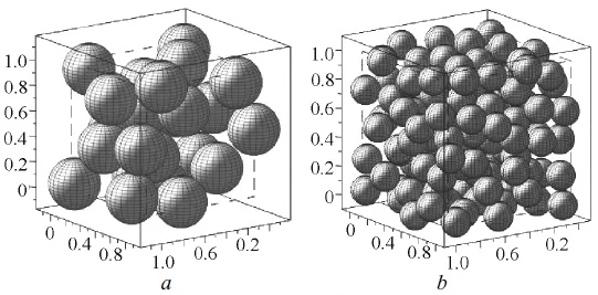
Two sphere packings of different radii when d = 3. The one on the left has a lower density than the one on the right.

It can be shown that we can swap the supremum and the limit in the definition of $\theta(d)$, and so we will be fixing an arbitrary cube $[-L, L]^d$ and maximizing the density of a packing $\mathcal{P} \subset [-L, L]^d$.

The Trivial Lower Bound

However, it is not known what the exact value of $\theta(d)$ is, and recent advancements have only been able to find the answer for $d = 1, 2, 3, 4, 8, 24$. So, we will instead focus on a trivial lower bound on $\theta(d)$ and try to find an algorithm for generating a packing that achieves this lower bound. Let $\mathcal{P}$ be a sphere packing that is maximal, i.e, adding another point $x$ into $\mathcal{P}$ will cause $x$ to be within distance $2r_d$ of some other point in $\mathcal{P}$. Consider a point $y \in [-L, L]^d$. We know that $\exists x \in \mathcal{P}$ such that $||x-y||_2 \leq 2r_d$ (otherwise, we could add $y$ to $\mathcal{P}$ and the packing is not maximal). But then, we know that $y \in B(x, 2r_d)$, where $B(x, 2r_d)$ is the ball centered at $x$ with radius $2r_d$. Since $y$ was arbitrary, observe that $\cup_{x \in \mathcal{P}} B(x, 2r_d)$ covers the entire cube $[-L, L]^d$. So, since the cube has volume $(2L)^d$, we can conclude $$ (2L)^d \leq \sum_{x \in \mathcal{P}} \text{vol}(B(x, 2r_d)) \leq 2^d \cdot |\mathcal{P}| $$ where the last step follows because $r_d$ was chosen such that the volume of a ball of radius $r_d$ is 1, so $\text{vol}(B(x, 2r_d)) = 2^d$. Rearranging, we see that $\frac{|\mathcal{P}|}{(2L)^d} \geq \frac{1}{2^d}$, and because $\mathcal{P}^d \subset [-L, L]^d$ we have that $\theta(d) \geq \frac{1}{2^d}$. But how can we actually generate a packing that achieves this lower bound?

Connections to Graph Theory

A breakthrough insight made my mathematicians was to recognize the connection between this problem and graph theory. Consider the following graph $G = (V, E)$ where $V \subseteq X \subseteq [-L, L]^d$ and $E = \{(x, y) \in V \times V \mid ||x-y||_2 < 2r_d\}$. Define an independent set in $G$ to be a set of vertices $I \subseteq V$ such that $(x, y) \notin E$ for all $x, y \in I$. Now, note that an independent set in $G$ corresponds to a sphere packing because if $(x, y) \not\in E$, then $||x-y||_2 \geq 2r_d$. So, the sphere packing problem is equivalent to finding the largest independent set in $G$. So now, we can rewrite $\theta(d)$ as $$ \theta(d) = \frac{\alpha(G)}{(2L)^d} $$ where $\alpha(G)$ is the size of the largest independent set in $G$.

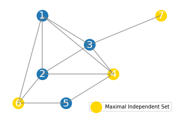
An example of a graph G and its largest independent set I.

Before we proceed further, note that for $G$ to exist, we need to find an $X$ that is finite. To do this, we will generate a set of random points in $[-L, L]^d$ such that $X$ is a realization of a poisson point process with intensity $\lambda$. This means that the expected number of points in $X$ is $\lambda \cdot \text{vol}([-L, L]^d) = \lambda \cdot (2L)^d$, and so $|X| \sim Po(\lambda \cdot (2L)^d)$.

Randomized Algorithm

An important result in graph theory is Turán's theorem, which states that for a graph $G$ with $\Delta$ such that $d(G) \geq \Delta$, then $\alpha(G) \geq \frac{|V|}{\Delta + 1}$, where $d(G)$ is the maximum degree of all vertices in $G$. We will use this theorem to come up with a randomized algorithm that achieves the trivial lower bound on $\theta(d)$. The algorithm is as follows:

1. Generate a realization of a poisson point process with large enough $\lambda$ in $[-L, L]^d$.
2. Construct the graph $G$ as described above, and choose $\Delta = \lambda \cdot 2^d$.
3. If $d(G) \geq \Delta$, then remove all vertices with degree greater than $\Delta$.
4. Find the largest independent set $I$ in the resulting graph (Note that this is an NP-hard problem, but runtime is for another post ...)
5. Return $I$ as $\mathcal{P}$.

If we can show that the deletion step, in expectation, does not remove too many points, then we can argue that the algorithm achieves the trivial lower bound on $\theta(d)$. By Turán's theorem, the size of the largest independent set in the graph outputted by the algorithm $\alpha(G) \geq \frac{|V|}{\Delta + 1},$ which in expectation is equal to $\frac{|X|}{\Delta + 1} = \frac{\lambda \cdot (2L)^d}{\lambda \cdot 2^d + 1} \geq \frac{(2L)^2}{2^d + 1} \geq \frac{(2L)^d}{2^d}$. Plugging this value in for $\alpha(G)$, we see that $\theta(d) \geq \frac{1}{2^d}$, achieving the trivial lower bound.

To see that the deletion step does not remove too many points, we can find the probability that a point $x \in X$ has degree greater than $\Delta$. This happens when $x$ is within distance $2r_d$ of more than $\Delta$ other points in $X$. Since $X$ is a realization of a poisson point process, the number of points in $X$ within distance $2r_d$ of $x$ is a poisson random variable with mean $\lambda \cdot \text{vol}(B(x, 2r_d)) = \lambda \cdot 2^d$. So, the probability that $x$ has degree greater than $\Delta$ is $$P(X \geq \Delta) = 1 - P(X < \Delta) = 1 - \sum_{i=0}^{\Delta - 1} \frac{e^{-\lambda \cdot 2^d} \cdot (\lambda \cdot 2^d)^i}{i!}$$

We can show that this probability is small for large enough $\lambda$ and $d$, and so the deletion step does not remove too many points in expectation.

Implementation

We will now implement the algorithm in Python and visualize the sphere packing generated by the algorithm.

import numpy as np
import math
import matplotlib.pyplot as plt
import networkx as nx
from networkx.algorithms import approximation as approx
from scipy.spatial import distance_matrix

class SpherePacking:
    def __init__(self, lambda_, L, d, r_d):
        self.lambda_ = lambda_
        self.L = L
        self.d = d
        self.r_d = r_d
        self.points = None

    def generate_poisson_points(self):
        num_points = np.random.poisson(self.lambda_ * (2 * self.L) ** self.d)
        return np.random.uniform(-self.L, self.L, size=(num_points, self.d))

    def construct_graph(self, points):
        distances = distance_matrix(points, points)
        adj_mat = (distances < 2 * self.r_d) & (distances > 0)
        return adj_mat

    def independent_set(self, adjacency_matrix):
        G = nx.Graph()
        num_vertices = adjacency_matrix.shape[0]
        G.add_nodes_from(range(num_vertices))
        for i in range(num_vertices):
            for j in range(i + 1, num_vertices):
                if adjacency_matrix[i, j]:
                    G.add_edge(i, j)
        return approx.maximum_independent_set(G)

    def pack(self):
        points = self.generate_poisson_points()
        adjacency_matrix = self.construct_graph(points)

        max_degree = int(self.lambda_ * (2 ** self.d))

        # Remove vertices whose degree is greater than max_degree
        degrees = adjacency_matrix.sum(axis=1)
        high_degree_mask = degrees > max_degree
        points = points[~high_degree_mask]
        adjacency_matrix = self.construct_graph(points)

        self.points = points[list(self.independent_set(adjacency_matrix))]

    def plot(self):
        fig = plt.figure()
        if self.d == 2:
            ax = fig.add_subplot(111)
            ax.set_xlim(-self.L, self.L)
            ax.set_ylim(-self.L, self.L)
            for point in self.points:
                circle = plt.Circle(point, self.r_d, color='red', alpha=0.3)
                ax.add_artist(circle)
            ax.scatter(self.points[:, 0], self.points[:, 1], color='blue', label='Circle Centers', s=2)
        elif self.d == 3:
            from mpl_toolkits.mplot3d import Axes3D
            ax = fig.add_subplot(111, projection='3d')
            ax.set_xlim(-self.L, self.L)
            ax.set_ylim(-self.L, self.L)
            ax.set_zlim(-self.L, self.L)
            ax.scatter(self.points[:, 0], self.points[:, 1], self.points[:, 2], color='blue', label='Sphere Centers', s=2)
            for point in self.points:
                u = np.linspace(0, 2 * np.pi, 20)
                v = np.linspace(0, np.pi, 20)
                x = self.r_d * np.outer(np.cos(u), np.sin(v)) + point[0]
                y = self.r_d * np.outer(np.sin(u), np.sin(v)) + point[1]
                z = self.r_d * np.outer(np.ones_like(u), np.cos(v)) + point[2]
                ax.plot_surface(x, y, z, color='red', alpha=0.3, edgecolor='none')
        else:
            raise ValueError("Cannot plot more than 3 dimensions")

        plt.legend()
        plt.show()

Let's visualize the 2D case first of the algorithm.

lambda_ = 10 # (For a denser packing, increase lambda_, but computation time will increase as well)
L = 10 # Length of the cube
d = 2 # Dimension of the space
r_d = math.gamma(d / 2 + 1) / (math.pi ** (d / 2)) ** (1 / d)  # Radius of the sphere with volume 1

sp_2d = SpherePacking(lambda_, L, d, r_d)
sp_2d.pack()
sp_2d.plot()

Now, let's plot the 3D case of the algorithm (with smaller $\lambda$ for computational reasons).

lambda_ = 1
L = 10
d = 3
r_d = math.gamma(d / 2 + 1) / (math.pi ** (d / 2)) ** (1 / d)

sp_3d = SpherePacking(lambda_, L, d, r_d)
sp_3d.pack()
sp_3d.plot()

Note that in both dimensions, the sphere packing generated is not optimal, but achieves the trivial lower bound on $\theta(d)$. To generate a more optimal packing, we need to simply choose a $\lambda$ that is large enough such that the probability that a point has degree greater than $\Delta$ is small. In a future post, maybe we can plot the density of the packing as a function of $\lambda$ and see how it changes.