Introduction
Drawing samples from a probability distribution \(\pi\) is a problem that arises often in computer science. For example in generative AI, language models sample tokens from learned probability distributions to generate new text. In computer graphics, many graphical engines randomly sample light paths bouncing around to simulate realistic lighting. But what exactly does it mean for a computer or an algorithm to sample from a probability distribution? How can a deterministic machine like a modern computer sample “randomly” from a distribution?
Hardware Assumptions
On most modern computers, one bit represents an atom of data or computation. So, if we want our computer to generate random samples, we would probably need it to be able to generate uniformly random bits. Let’s assume we have a black box machine that does exactly that.
Above assumption is not an unrealistic one since we have hardware random bit generators which generate random bits from physical process that produce entropy.
More formally, let \(B \in \{0, 1\}\) be a uniform random bit with \[\mathbb{P}[B = 0] = \mathbb{P}[B = 1] = \frac{1}{2}\] and assume that we can sample from \(B\).
The Uniform Distribution
Let’s start the discussion by coming up with algorithms for sampling integers uniformly randomly in a fixed range.
Integer in range \([0, 2^N]\)
First, let’s see if we can generate a uniformly random integer \(M \in \{0, \cdots, 2^N - 1\}\). That is, we want to come up with an algorithm to produce \(M\) such that \[\mathbb{P}[M = m] = \frac{1}{2^N}\] for all \(m \in \{0, \cdots, 2^N - 1\}\).
Well, given that we only have a random bit generator, there is really only one thing we can do here. We should generate \(N\) independent bits using our random bit generator and concatenate them together to get the base 2 representation of the integer we return.
Algorithm 1
\(M \gets 0\)
for \(i = 1\) to \(N\) do
\(\quad M \gets M + B_i \cdot 2^i\)
return \(M\)
Let’s check that this gives us the desired result. Let \(B_1, B_2, \dots, B_N\) be the bits we generated. Now, note that for any integer \(k \in \{0, \cdots, 2^N - 1\}\), there exists a unique binary representation: \[ k = \sum_{i = 1}^{N} b_i \cdot 2^i \] where each \(b_i \in \{0, 1\}\) is the \(i\)-th bit of \(k\). The probability that \(M = k\) is given as: \[\begin{align*} \mathbb{P}[M = k] &= \mathbb{P}[B_0 = b_0, B_1 = b_1, \cdots, B_n = b_n] \\ &= \mathbb{P}[B_0 = b_0] \cdot \mathbb{P}[B_1 = b_1] \cdots \mathbb{P}[B_N = b_n] \tag{By independence} \\ &= \frac{1}{2} \cdot \frac{1}{2} \cdots \frac{1}{2} \tag{$N$ times} \\ &= \frac{1}{2^N} \end{align*}\] as desired.
Integer in Arbitrary Range
Great, now lets move onto a slightly more difficult problem: generating a uniformly random integer in \(\{0, \dots, M\}\), where \(M\) is not necessarily a power of \(2\).
A first idea would be to use the same approach as before and concatenate a string of \(N\) random bits. This, however, does not work. For example, if \(N = 3\) and \(M = 4\) then our random bit generator produces outcomes in the range \(\{0, \dots, 2^3 - 1\} = \{0, 1, 2, 3, 4, 5, 6, 7\}\). Each of these \(8\) outcomes occurs with probability \(\frac{1}{8}\). However, we wanted an integer in the range \(\{0, 1, 2, 3, 4\}\), and the probability of each outcome to be exactly \(\frac{1}{5}\).
Another approach would be to generate \(N\) random bits as before, and then return \(N \mod (M + 1)\). I leave it as an exercise to figure out why this approach also does not work (Hint: use the same counter example from above).
Notice that the issue in the above two approach is that our algorithm considers values that are outside the given range. To fix this problem, one idea would be to simply ignore an integers that are outside the range. More formally, define the algorithm as
Algorithm 2
\(P \gets \lceil \log_2 (M + 1) \rceil\)
repeat
\(\quad\) Generate \(N \in \{0, \cdots, 2^P - 1\}\) using Algorithm 1
until \(N \leq M\)
return \(N\)
This algorithm is called rejection sampling. A subtle difference between this algorithm and the previous algorithm is that its running time is non-deterministic. For example, we know that algorithm 1 terminates after generating \(N\) random bits. Algorithm 2, however, has no such guarantees. It is technically possible that we get really really really unlucky and always generate \(N > M\) and so the algorithm would never return a number.
So, let’s compute probability that the algorithm terminates, which only happens when \(N \leq M\) \[\begin{align*} \mathbb{P}[N \leq M] &= \sum_{i \leq M} \mathbb{P}[N = i] \tag{CDF of $N$} \\ &= \sum_{i = 0}^M \frac{1}{2^N} \tag{From Algorithm 1} \\ &= \frac{(M + 1)}{2^N} \end{align*}\]
Note that if \(M \ll N\) then the exponential in the denominator dominates, and the probability of terminating is near zero. When \(M \gg N\) then the fraction is approximately linear, and so the algorithm terminates with higher probability.
However, in the case that the algorithm does return, then we can be sure that it is correct. We prove this below. Note that for any \(k \in \{0, \cdots, M\}\), we have \[\begin{align*} \mathbb{P}[N = k] &= \mathbb{P}[N = k | N \leq M] \tag{Since $N \leq M$ iff $N$ is returned} \\ &= \frac{\mathbb{P}[N = k, N \leq M]}{\mathbb{P}[N \leq M]} \tag{Definition of conditional prob.} \\ &= \frac{\mathbb{P}[N = k]}{\mathbb{P}[N \leq M]} \tag{$k \leq M$ so if $N = k$, we know $N \leq M$} \\ &= \frac{1/2^N}{(M+1)/2^N} \\ &= \frac{1}{M + 1} \end{align*}\] as desired.
Real number in range \([0, 1]\)
Now let’s move onto the hardest problem yet: sampling a real number in the range \([0, 1]\). Note that every real number \(r \in [0, 1]\) can be represented as a binary expansion: \[ r = \sum_{i=1}^{\infty} \frac{B_i}{2^i} = 0.B_1B_2B_3\dots \] where each \(B_i \in \{0, 1\}\). Again, our first instinct should be to ask if generating an infinite string of bits and concatenating them gives us the desired result. In this case, it turns out to be true. However, the proof of this fact is non-trivial and takes quite a lot of work.
If \(B_1, B_2, B_3, \dots\) are independent uniform random bits, then \[ U = \sum_{i=1}^{\infty} \frac{B_i}{2^i} \] is uniformly distributed on \([0, 1]\).
To prove this, we need to show that for any interval \([a, b) \subseteq [0, 1]\), we have \[ \mathbb{P}[U \in [a, b)] = \text{length}([a, b)]) = b - a \]
Partitioning \([0, 1]\) and characterizing the partitions
The proof uses a clever partitioning argument. We’ll divide \([0, 1]\) into dyadic intervals, which are defined to be intervals whose endpoints are fractions with powers of 2 in the denominator.
For any arbitrary \(k \in \mathbb{N}\), we can partition \([0, 1]\) into \(2^k\) equal intervals: \[ I_j = \left[\frac{j}{2^k}, \frac{j+1}{2^k}\right) \quad \text{for } j = 0, 1, \dots, 2^k - 1 \]
Each interval has length \(\frac{1}{2^k}\), and together they cover the entire unit interval. The larger \(k\), the better this approximation gets.
Now, I claim that the first \(k\) bits \((B_1, \dots, B_k)\) of \(U\) completely determine which dyadic interval \(I_j\) contains the value \(U\). Specifically: \[ U \in I_j = \left[\frac{j}{2^k}, \frac{j+1}{2^k}\right) \iff \sum_{i=1}^{k} \frac{B_i}{2^{i}} = \frac{j}{2^k} \]
To see why, we can decompose \(U\) into two parts:
\[ U = \underbrace{\sum_{i=1}^{k} \frac{B_i}{2^i}}_{:=U_k} + \underbrace{\sum_{i=k+1}^{\infty}\frac{B_i}{2^i}}_{:=R_k} \] where \(U_k\) represents the first \(k\) bits and \(R_k\) represents the remaining bits. Now, note that The first \(k\) bits can only produce discrete values because there are \(2^k\) possible bit strings of length \(k\), and these values are \[\left\{0, \frac{1}{2^k}, \frac{2}{2^k}, \ldots, \frac{2^k-1}{2^k}\right\}\] Observe that these are exactly the left endpoints of our dyadic intervals \(I_j\).
Now, The remaining bits \(R_k\) can be rewritten by factoring out \(\frac{1}{2^k}\): \[\begin{align*} R_k &= \sum_{i=k+1}^{\infty} \frac{B_i}{2^i} = \frac{1}{2^k} \sum_{i=1}^{\infty} \frac{B_{k+i}}{2^i} \end{align*}\] Since \(\sum_{i=1}^{\infty} \frac{B_{k+i}}{2^i}\) is a binary expansion taking values in \([0, 1)\), we have \[0 \leq R_k < \frac{1}{2^k}\] So, we have that \(R_k\) is strictly less than the width of a dyadic interval.
Therefore, we can now claim that if \(U_k = \frac{j}{2^k}\), then \(U = \frac{j}{2^k} + R_k\) must satisfy \[\frac{j}{2^k} \leq U < \frac{j+1}{2^k}\] placing \(U\) in interval \(I_j\). Conversely, if \(U \in I_j\), the constraint \[\frac{j}{2^k} \leq U < \frac{j+1}{2^k}\] combined with the fact that \(U_k\) is a discrete value in this range forces \(U_k = \frac{j}{2^k}\). Therefore, we have shown that
Probability of landing in \(I_j\)
Now we can calculate the probability that \(U\) lands in a specific dyadic interval \(I_j\):
\[\begin{align*} \mathbb{P}[U \in I_j] &= \mathbb{P}\left[\sum_{i=1}^{k} \frac{B_i}{2^{i}} = \frac{j}{2^k}\right] \\ &= \mathbb{P}[B_1 = b_1, B_2 = b_2, \dots, B_k = b_k] \end{align*}\]
where \((b_1, \dots, b_k)\) is the binary representation of \(j\).
Since the bits are independent and each has probability \(\frac{1}{2}\):
\[\begin{align*} \mathbb{P}[U \in I_j] &= \prod_{i=1}^{k} \mathbb{P}[B_i = b_i] \\ &= \prod_{i=1}^{k} \frac{1}{2} \\ &= \frac{1}{2^k} \end{align*}\]
Note that this is exactly the length of the interval \(I_j\)! Therefore, we have show that at least for dyadic intervals, \(U\) is uniformly distributed!
Extending to General Intervals
Extending this to the general interval \([a, b]\) is complicated and requires careful machinery taught usually in a course in real analysis. Therefore, will handwave a lot of the technicalities, but do keep in mind that there is more careful argument to be made here.
For a general interval \([a, b) \subseteq [0, 1]\), we approximate it using dyadic intervals. Let \(J_k\) be the set of indices where \(I_j \subseteq [a, b)\). Then:
\[ [a, b) \approx \bigcup_{j \in J_k} I_j \]
As \(k\) increases, the dyadic intervals become finer, and this approximation improves.
Since the dyadic intervals are disjoint:
\[\begin{align*} \mathbb{P}\left[U \in \bigcup_{j \in J_k} I_j\right] &= \sum_{j \in J_k} \mathbb{P}[U \in I_j] \\ &= \sum_{j \in J_k} \frac{1}{2^k} \\ &= \frac{|J_k|}{2^k} \end{align*}\]
where \(|J_k|\) is the number of dyadic intervals that fit inside \([a, b)\).
Taking the Limit
Notice that \(\frac{|J_k|}{2^k}\) represents the total length of all dyadic intervals contained in \([a, b)\):
\[ \frac{|J_k|}{2^k} = \sum_{j \in J_k} \text{length}(I_j) \]
As \(k \to \infty\), these intervals cover \([a, b)\) with increasing precision, so we expect
\[ \lim_{k \to \infty} \frac{|J_k|}{2^k} = b - a \]
Therefore:
\[\begin{align*} \mathbb{P}[U \in [a, b)] &= \lim_{k \to \infty} \mathbb{P}\left[U \in \bigcup_{j \in J_k} I_j\right] \\ &= \lim_{k \to \infty} \frac{|J_k|}{2^k} \\ &= b - a \\ &= \text{length}([a, b)) \end{align*}\]
as desired
From Theory to Practice: Finite Bit Algorithms
The theoretical result above is beautiful, but it has a glaring practical issue: we cannot generate an infinite sequence of bits! In the real world, we need to work with a finite number of bits. Fortunately, our proof gives us a natural way to approximate the uniform distribution using only a finite number of bits.
The key insight is that after generating \(N\) bits, we’ve already determined which of the \(2^N\) dyadic intervals our value falls into. The remaining (ungenerated) bits would only refine our position within that interval, which has width \(\frac{1}{2^N}\). For large \(N\), this interval is so small that the difference is negligible
This leads us to the following algorithm:
Algorithm 3
\(U \gets 0\)
for \(i = 1\) to \(N\) do
\(\quad\) Generate random bit \(B_i\)
\(\quad\) \(U \gets U + B_i \cdot 2^{-i}\)
return \(U\)
This algorithm generates values of the form \(\frac{k}{2^N}\) where \(k \in \{0, 1, \ldots, 2^N - 1\}\). In other words, it produces a discrete uniform distribution over \(2^N\) equally-spaced points in \([0, 1]\), rather than a truly continuous uniform distribution.
Let \(U_N\) denote the output of Algorithm 3 and let \(U_{\text{true}}\) denote a truly uniform random variable on \([0, 1]\). How far off is our approximation? Well the maximum distance between any generated value and its “true” counterpart is at most the granularity of our discretization: \[ \max_{x \in [0, 1]} |U_N - x| \leq \frac{1}{2^N} \] So, if \(N = 64\), then we have: \[\begin{align*} \frac{1}{2^{64}} &\approx 5.42 \times 10^{-20} \\ \end{align*}\]
This means our approximation error is about \(10^{-20}\)! For all practical purposes, this is indistinguishable from a true uniform distribution. In fact, 64-bit floating point numbers (the standard in most programming languages) have a precision of about \(10^{-16}\), which is less precise than our sampling error.
In practice, most programming languages use 64-bit floating point numbers for representing real numbers. Algorithm 3 with \(N = 64\) bits produces values that are uniformly distributed on the set of representable floating point numbers in \([0, 1]\), which is the best we can do given the finite precision of computer arithmetic.
Therefore, Algorithm 3 with \(N = 64\) bits gives us an excellent practical algorithm for sampling (approximately) uniform real numbers in \([0, 1]\).
Arbitrary Probability Distribution
That was a lot of work! If it took so much effort just to sample from the uniform distribution, how can we possibly expect to come up with algorithms for complicated probability distributions? Well, it turns out that with not too much extra work we can sample from any arbitrary distribution \(\pi\). More formally, lets say \(\pi\) is a probability distribution on a finite state space \(\chi = \{x_1, \cdots x_n\}\). I want to generate an \(X \in \chi\) such that \[ \mathbb{P}[X = x] = \pi(x) \] Now that we can sample from the uniform distribution on \([0, 1]\), let’s use that. We will use another clever partitioning technique, similar to what we did for proving the uniform distribution result.
More specifically, we divide the interval \([0, 1]\) into \(N\) consecutive segments. For each \(i \in \{1, 2, \ldots, N\}\), define segment \(i\) as: \[ S_i = \left[\sum_{j=1}^{i-1} \pi(x_j), \sum_{j=1}^{i} \pi(x_j)\right) \] where by convention, \(\sum_{j=1}^{0} \pi(x_j) = 0\).
Observe that segment \(S_i\) has length: \[ \text{length}(S_i) = \sum_{j=1}^{i} \pi(x_j) - \sum_{j=1}^{i-1} \pi(x_j) = \pi(x_i) \]
Moreover, these segments partition \([0, 1]\) since they are disjoint and: \[ \bigcup_{i=1}^{N} S_i = [0, 1) \] which follows from the fact that \(\sum_{i=1}^{N} \pi(x_i) = 1\) (since \(\pi\) is a probability distribution). When we sample uniformly from \([0, 1]\), the probability of landing in segment \(i\) is exactly \(\pi(x_i)\) (since the segment has length \(\pi(x_i)).\) So if we return \(x_i\) whenever we land in segment \(i\), we get the desired distribution!
Think of it like a dartboard: if you throw a dart uniformly at random on \([0,1]\), the probability of hitting a region is proportional to its length. By making segment \(i\) have length \(\pi(x_i)\), we ensure the probability of hitting it matches our target probability.
Example: Suppose \(\mathcal{X} = \{x_1, x_2, x_3, x_4, x_5\}\) and \(\pi = (0.15, 0.25, 0.20, 0.30, 0.10)\). We segment the \([0, 1]\) interval as shown below:
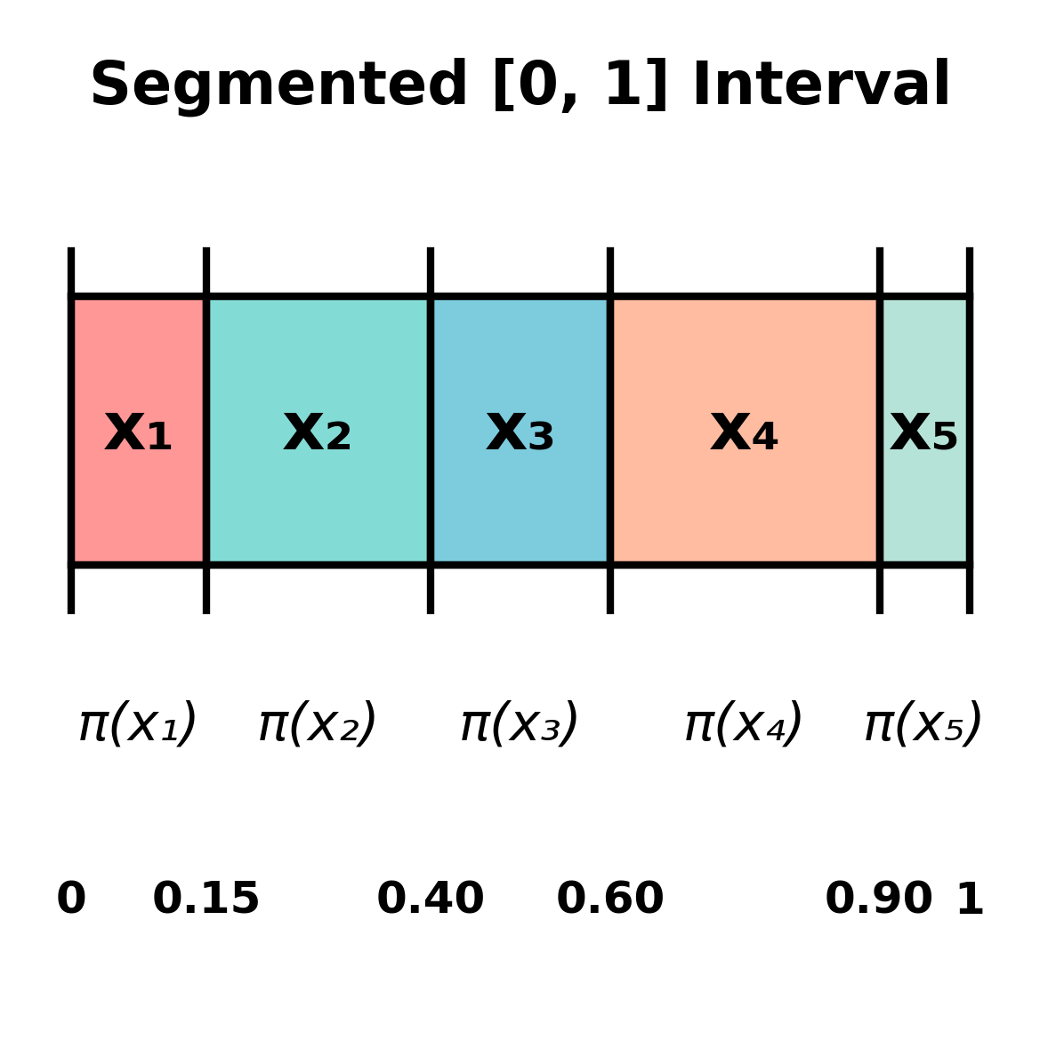
Now, we can sample a real number uniformly random, and return the segment that this number belongs to.
Formalizing the Algorithm
To implement this efficiently, we use cumulative probabilities. Define: \[ F_i = \sum_{j=1}^{i} \pi(x_j) \quad \text{for } i = 1, 2, \ldots, N \] with \(F_0 = 0\). Note that \(F_i\) represents the cumulative probability up to and including \(x_i\), so segment \(i\) corresponds to the interval \([F_{i-1}, F_i)\).
Our algorithm returns \(x_i\) when \(U\) falls in the interval \([F_{i-1}, F_i)\):
Algorithm 4
Preprocessing:
Compute cumulative probabilities: \(F_0 \gets 0\)
for \(i = 1\) to \(N\) do
\(\quad\) \(F_i \gets F_{i-1} + \pi(x_i)\)
Sampling:
Generate \(U \sim \text{Uniform}[0, 1]\) using Algorithm 3
for \(i = 1\) to \(N\) do
\(\quad\) if \(F_{i-1} \leq U < F_i\) then
\(\quad\quad\) return \(x_i\)
Let’s verify that this algorithm produces the correct distribution. For any \(x_i \in \mathcal{X}\):
\[\begin{align*} \mathbb{P}[\text{output} = x_i] &= \mathbb{P}[F_{i-1} \leq U < F_i] \\ &= F_i - F_{i-1} \tag{$U$ is uniform on $[0,1]$} \\ &= \left(\sum_{j=1}^{i} \pi(x_j)\right) - \left(\sum_{j=1}^{i-1} \pi(x_j)\right) \\ &= \pi(x_i) \end{align*}\]
The second equality uses the fact that for a uniform random variable \(U\) on \([0,1]\), we have \(\mathbb{P}[a \leq U < b] = b - a\). Therefore, our algorithm produces samples distributed according to \(\pi\). Problem solved!
The preprocessing step takes \(O(N)\) time to compute cumulative probabilities. Each sample then requires \(O(N)\) time in the worst case to find which segment \(U\) falls into (via linear search). This can be improved to \(O(\log N)\) per sample using binary search, since the cumulative probabilities \(F_i\) are sorted.