Introduction
In a previous blog post, I discussed various algorithms for sampling from a probability distribution \(\pi\). These algorithms all made a simple assumption: we can compute \(\pi(x)\) efficiently for all \(x\) in our sample space \(\chi\). However, this assumption might be too strong for certain cases. What if computing \(\pi(x)\) is computationally intractable? We can’t use the methods developed in that post. What do we do instead?
Protein Folding
As an example of a situation where \(\pi\) is uncomputable, let’s study protein folding. You might recall that a protein is a chain of amino acids (also called residues) that folds into a certain structure. One of the simplest models for this process is the Hydrophobic-Polar (HP) lattice model, where we have a chain of \(N\) residues, each classified as either hydrophobic (H) which is water-repelling, or polar (P) which is water-loving. Chemistry tells us that hydrophobic residues tend to cluster together, and so the final folded structure of an acid sequence is heavily influenced by \(H\) and \(P\) residues. We can see this effect in the diagram below:
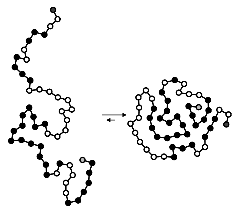
On the left is an unfolded amino acid sequence, with hydrophobic residues in black and polar particles in white. Observe that after folding, the hydrophobic residues clustered together on the “inside” of the protein, while the polar residues are closer to the surface of the protein.
Mathematically, the folded structure of this amino acid can be modeled as a graph on a 2D integer lattice where each residue is mapped to a point in space. However, we can’t just consider any arbitrary graph. To keep this model realistic, we need to have the restriction that adjacent amino acids in the sequence are adjacent in the lattice (since the amino acid sequence cannot be permuted when folding), and no two residues occupy the same point in space. We can define this more formally as follows:
An amino acid sequence is a string \(s \in \{H, P\}^N\) of length \(N\). A folded configuration of this sequence is a function \(\omega : [1, \cdots, N] \to \mathbb{Z}^2\) where \(\omega(i)\) gives the position of the \(i\)-th amino acid in \(s\) on the lattice, such that
- \(||\omega(i) - \omega(i+1)||_2 = 1\) for all \(1 \leq i < N\) (adjacent residues in the sequence are adjacent in the lattice)
- \(\omega(i) \neq \omega(j)\) for all \(i \neq j\) (two residues cannot occupy the same point in space)
Chemistry tells us that the energy of a configuration \(\omega\) depends on hydrophobic contacts. We say two residues at positions \(\omega(i)\) and \(\omega(j)\) are in contact if they are adjacent on the lattice but not consecutive in the sequence so that \(|i−j| > 1\). This way, we only count the interactions of residues that moved around in 2D space to cluster together, rather than ones that were already next to each other. The energy is then: \[E(s, \omega) = \sum_{i \sim j} E_{s_i, s_j}\] where \(i \sim j\) iff \(\omega(i)\) is in contact with \(\omega(j)\), and \(E_{HH} = -1\), \(E_{HP} = E_{PH} = E_{PP} = 0\), so only \(HH\) contacts contribute to lowering the energy, and giving us a way to quantify the clustering behavior of \(H\) residues.
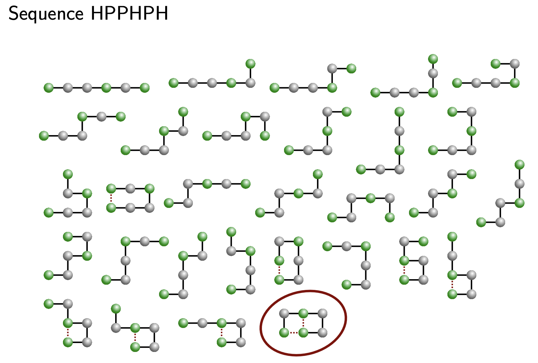
Below is an example sequence \(HPPHPH\) and possible folded configurations \(\omega\). \(H\) amino acids are colored green and \(P\) amino acids are in silver. The configuration \(\omega\) that has the minimum energy of all the listed configurations is circled in red, since it has three \(HH\) contacts, most out of the others. Image courtesy of MIT: 18.417
Given this set up, our goal is to study the folded protein structure of an amino acid sequence. Specifically, we want to understand what a typical folded configuration looks like at temperature \(T\). Thermochemistry tells us that protein folding can actually be thought of sampling from a distribution proportional to the Boltzmann distribution: \[ \pi_u(\omega | s) := \mathbb{P}[\omega | s] = e^{-\frac{E(s, \omega)}{k_B T}} \] where \(T\) is the temperature, \(k_B\) is the Boltzmann constant. To turn \(\pi_u\) into a probability distribution, we need to compute a normalizing constant \[ Z = \sum_{\omega}\pi_u(\omega | s) \] and define \[ \pi(\omega | s) := \frac{1}{Z} \pi_u (\omega | s) \]
We can now use the algorithm developed at the end of this post to draw samples from this distribution and understand what typical folded protein configurations look like at temperature \(T\). There’s just one problem: the normalizing constant \(Z\).
Intractability of \(Z\)
We need to compute \(\pi_u(\omega | s)\) for all possible \(\omega\) given a specific \(s\) to find \(Z\). What could happen if the number of possible configurations is computationally intractable? In this case, it turns out that there are about \(3^N\) different \(\omega\)’s. This is because we can place the first residue anywhere on the lattice, and so the second residue has \(4\) choices (up, down, left, right). The third residue has at most three choices (since we can’t backtrack to residue \(1\)’s position), and similarly with the fourth residue. We can continue this argument for \(N\) and get the rough bound \(3^N\) for the number of possible configurations.
This is a huge number! Even if we have a relatively small amino acid sequence, with \(N = 100\), there are roughly \(3^{100}\) possible configurations to try! Even our fastest computers today will take about \(10^{22}\) years to finish calculating that a sum of that many terms. What’s worse is that there is no smarter way to compute \(Z\). We need to evaluate \(\pi_u\) at every single \(\omega\). This makes it impossible to use our previously developed algorithms since it is hopeless to try to compute \(\pi (\omega | s)\). We need to think of another way to solve this problem.
If we can’t compute \(\pi(\omega | s)\) directly, are there quantities that we can compute? Well, we can evaluate \(\pi_u (\omega | s)\) since that just requires counting the \(HH\) contacts for a single \(\omega\). Does this help us come up with a way to understand how \(\pi\) looks like? Suppose we have two configurations, \(\omega\) and \(\omega'\). While we don’t know their individual probabilities \(\pi(\omega | s)\) or \(\pi(\omega' | s)\), observe what happens when we look at their ratio:
\[ \frac{\pi(\omega' | s)}{\pi(\omega | s)} = \frac{\pi_u(\omega' | s)/Z}{\pi_u(\omega | s)/Z} = \frac{\pi_u(\omega' | s)}{\pi_u(\omega | s)} \]
The \(Z\) terms cancel out entirely. We are left with a ratio of unnormalized weights (\(\pi_u\)), which is just a simple calculation of \(HH\) contacts. Now, notice that the fraction
\[ \frac{\pi(\omega' | s)}{\pi(\omega | s)} \]
tells us the relative probability of two configurations. If this ratio is greater than \(1\), then \(\omega'\) has higher probability than \(\omega'\). If it’s less than \(1\) then \(\omega\) has higher probability. Using this, we can compare the likelihood of two configurations.
This should hopefully give you an idea. Since we can’t look at the whole landscape of \(3^N\) configurations to pick a perfect sample, we start with a single, arbitrary configuration \(\omega_0\). It’s almost certainly not a typical sample from \(\pi\), but that doesn’t matter yet. We want to produce a sequence of configurations \(\omega_0, \omega_1, \omega_2, \dots, \omega_t\) such that, as \(t \to \infty\), the configurations look less like our arbitrary start and more like they were drawn from \(\pi\). To do this, at each step \(t\), we should propose a new candidate \(\omega'\). Then, we should decide if we should update our current sample to \(\omega'\), or keep \(\omega_t\) as the candidate. But how do we make this decision?
Hopefully you see that we can use our ratio \[\frac{\pi(\omega' | s)}{\pi(\omega_t | s)}\] as a way to filter. If the ratio is high, \(\omega'\) is more likely than our current state. We should probably update our sample to \(\omega'\). If the ratio is low, it means \(\omega'\) is less likely. We should probably reject it and keep \(\omega_t\) as our sample for this step.
While our initial choice \(\omega_0\) might be a bad representative of the distribution, the process is self-correcting. Each time we make an update, we are moving the sequence toward states that is more representative under \(\pi\). If we run this process for long enough, the first arbitrary choice \(\omega_0\) gets drowned out. Eventually, the configurations the algorithm visits become more and more like they are samples drawn from the true distribution \(\pi\).
It turns out that \(\omega_t\) defined in this way is a Markov Chain. If you are unfamiliar with Markov Chains, I highly suggest you read my previous blog post on them. Be warned: the rest of this posts assumes you are familiar with the big ideas/theorems from that post!
The Metropolis-Hastings Algorithm
Note: From here on, I’ll remove the dependence on \(s\) for notational clarity, writing \(\pi(\omega)\) instead of \(\pi(\omega | s)\).
Notice that the process discussed at the end of the previous section can be thought of as a Markov Chain. We start out with some initial configuration \(\omega_0\), and for each time step decide if we need to resample an \(\omega_1\) or not. If we keep running this process, we’ll have a Markov Chain \(\omega_t\). I’ll leave it as an exercise for you to prove that this process indeed does have the Markov Property.
To turn this self-correcting sequence idea into an algorithm, we need to formalize how we pick a new candidate and how we decide to accept it.
First, we need a way to pick a candidate \(\omega'\) given our current state \(\omega_t\). We call this the proposal distribution, denoted \(Q(\omega' | \omega_t)\). In the case of our protein lattice, a proposal might be as simple as picking one residue at random and try to move it to an adjacent empty spot. This is just a mechanism to explore the space; \(Q\) doesn’t need to know anything about the \(HH\) contacts or the true distribution \(\pi\).
Once we have our candidate \(\omega'\), we need an exact rule for the filter. We want this rule to guarantee that the stationary distribution of our chain is exactly \(\pi\). This rule is the Acceptance Probability, \(\alpha(\omega_t, \omega')\). It tells us the exact probability with which we should move to the new state. If we don’t move, we simply stay at \(\omega_t\) for another time step.
Combining the ideas gives us the Metropolis-Hastings algorithm
Metropolis-Hastings Algorithm
\(\omega_0 \gets\) initial configuration
for \(t = 0\) to \(T-1\):
\(\quad\) Propose a new configuration \(\omega'\) with probability \(Q(\omega_t, \omega')\)
\(\quad\) Define the Acceptance Probability \(A(\omega_t, \omega')\) by:
\[ A(\omega_t, \omega') := \min\left\{1, \frac{\pi_u(\omega')Q(\omega', \omega_t)}{\pi_u(\omega_t)Q(\omega_t, \omega')}\right\} \] \(\quad\) Choose \(U_{t + 1} \sim \text{Unif}([0, 1])\) independently and update
\[ \omega_{t + 1} = \begin{cases} \omega' && \text{if } U_{t+1} \leq A \\ \omega_t && \text{otherwise}\\ \end{cases} \]
Note: \(T\) should be chosen large enough for the chain to reach its stationary distribution.
This algorithm is a more formal version of the intuition we’ve developed so far. It defines a new Markov Chain \(\omega_t\) (called the MH chain) and simulates this chain for a very long time.
But is this method actually correct? That is, will our sequence \(\omega_0, \omega_1, \cdots, \omega_t, \omega_{t + 1}, \cdots\) eventually look like it resembles \(\pi\) if we follow this algorithm? Well, we have a nice theorem (discussed in this post) that says irreducible and aperiodic Markov chains converge to their stationary distribution, no matter the starting distribution. So, if we can show that \(\pi\) is a stationary distribution of \(\omega_t\), and \(\omega_t\) is irreducible and aperiodic, then we can apply the theorem to conclude that \[ \lim_{t \to \infty} \mathbb{P}[\omega_t = \omega] = \pi(\omega) \]
The hard part in this is showing that \(\pi\) is indeed a stationary distribution of \(\omega_t\). There are some useful propositions we should prove first, to help us establish this result.
If \(\mu\) is a distribution and \(P\) is the transition matrix of a Markov Chain such that \[ \mu(x) P(x, y) = \mu(y) P(y, x) \] for every \(x, y \in \chi\), then \(\mu\) must be a stationary distribution of \(P\).
Proof:
Note that we have \[\begin{align*} (\mu P) (y) &= \sum_{x \in \chi}\mu(x) P(x, y) \\ &= \sum_{x \in \chi} \mu(y) P(y, x) \tag{By assumption}\\ &= \mu(y)\sum_{x \in \chi} P(y, x) \\ &= \mu(y) \tag{Since rows of $P$ sum to 1} \end{align*}\] Therefore, \(\mu\) is a stationary distribution.
Now, we can prove our correctness theorem:
The MH Markov Chain \(\omega_t\) as defined above has \(\pi\) as a stationary distribution.
Proof:
Note: Since ratios \(\pi(\omega') / \pi(\omega)\) equal \(\pi_u(\omega')/ \pi_u(\omega)\), the acceptance probabilities computed with \(\pi_u\) in the algorithm is equivalent to those computed with \(\pi\). Therefore, we can write the proof using \(\pi\) without loss of generality
First we need to identify the transition matrix of the Markov Chain \(\omega_t\). Observe that for any two configurations \(\omega\) and \(\omega'\), if \(\omega \neq \omega'\), then the probability that \(\omega_t\) transitions from \(\omega\) to \(\omega'\) is \(Q(\omega, \omega')A(\omega, \omega')\) since we propose \(\omega'\) independently and accept \(\omega'\) independently. Now, if \(\omega = \omega'\), then the probability that \(\omega_t\) transitions from \(\omega\) to \(\omega'\) is same as the probability that we do not make a transition at all. This is \[ 1 - \sum_{\omega'' \neq \omega} Q(\omega, \omega'') A(\omega, \omega'') \] Therefore, the transition matrix of the MH chain is given by \[ P(\omega, \omega') = \begin{cases} Q(\omega, \omega') A(\omega, \omega') && \text{if } \omega \neq \omega' \\ 1 - \sum_{\omega'' \neq \omega} Q(\omega, \omega'') A(\omega, \omega'') && \text{if } \omega = \omega' \end{cases} \]
Now, if \(\omega = \omega'\) then we trivially have the condition \[\begin{align*} \pi(\omega) P(\omega, \omega') &= \pi(\omega') P(\omega', \omega) \end{align*}\]
Therefore, by proposition \(1\), we can conclude that \(\pi\) is a stationary distribution of \(P\) in this case. Now, assume that \(\omega \neq \omega'\), and WLOG (by symmetry) that
\[\begin{align*} \pi(\omega) Q(\omega, \omega') &\leq \pi(\omega') Q(\omega', \omega) \\ 1 &\leq \frac{\pi(\omega') Q(\omega', \omega)}{\pi(\omega) Q(\omega, \omega')} \tag{All terms are non-negative} \end{align*}\]
This must imply that in this case, \[\begin{align*} A(\omega, \omega') &= \min\left\{1, \frac{\pi(\omega') Q(\omega', \omega)}{\pi(\omega) Q(\omega, \omega')}\right\} = 1 \end{align*}\]
Additionally, we must have \[ \begin{align*} A(\omega', \omega) &= \min\left\{1, \frac{\pi(\omega) Q(\omega, \omega')}{\pi(\omega') Q(\omega', \omega)}\right\} = \frac{\pi(\omega) Q(\omega, \omega')}{\pi(\omega') Q(\omega', \omega)} \end{align*} \] Now, we can put everything together and conclude that \[ \begin{align*} \pi(\omega)P(\omega,\omega') &= \pi(\omega)[Q(\omega,\omega')\underbrace{A(\omega,\omega')}_{=1} ] \\ &= \pi(\omega) Q(\omega,\omega') \\ \end{align*} \]
But we can also write:
\[ \begin{align*} \pi(\omega')P(\omega',\omega) &= \pi(\omega') Q(\omega',\omega)A(\omega',\omega) \\ &= \pi(\omega') Q(\omega', \omega) \left[\frac{\pi(\omega) Q(\omega, \omega')}{\pi(\omega') Q(\omega', \omega)}\right] \\ &= \pi(\omega) Q(\omega, \omega') \end{align*} \] Therefore, we have that \[ \pi(\omega)P(\omega,\omega') = \pi(\omega')P(\omega',\omega) \]
and so using proposition \(1\), we can conclude that \(\pi\) is in-fact a stationary distribution of \(P\). The other case is symmetric, and so this completes the proof.
Now, all that remains to prove correctness and gain apply the limiting theorem of Markov Chains and stationary distribution is to show that the MH chain is irreducible and aperiodic.
If the proposal distribution \(Q\) satisfies \(Q(\omega, \omega') > 0\) for all \(\omega, \omega' \in \chi\), then the MH chain is irreducible and aperiodic.
Proof:
Irreducibility: We need to show that for any two configurations \(\omega\) and \(\omega'\), there exists some \(t\) such that \(P^t(\omega, \omega') > 0\), meaning we can reach \(\omega'\) from \(\omega\) in finitely many steps.
Since \(Q(\omega, \omega') > 0\) by assumption, we can propose \(\omega'\) from \(\omega\) with positive probability. The acceptance probability satisfies \(A(\omega, \omega') > 0\) whenever \(Q(\omega, \omega') > 0\) since we’ve shown in the previous post that \(\pi > 0\) and we assumed that \(Q > 0\). Therefore, \[ P(\omega, \omega') = Q(\omega, \omega') A(\omega, \omega') > 0 \] This means we can reach any state from any other state in one step, making the chain irreducible.
Aperiodicity: Recall that a chain is aperiodic if for some state \(\omega\), we have \(\gcd\{t : P^t(\omega, \omega) > 0\} = 1\).
Notice that there is always a positive probability of rejecting the proposed state and staying at \(\omega\). Specifically, the probability of staying at \(\omega\) is at least the probability of proposing some \(\omega'\) and then rejecting it. Since there always exists some \(\omega'\) such that \(A(\omega, \omega') < 1\), we have \[ P(\omega, \omega) \geq Q(\omega, \omega') (1 - A(\omega, \omega')) > 0 \] for some \(\omega'\). This means we can return to \(\omega\) in one step with positive probability, which immediately implies the chain is aperiodic (since \(\gcd\) of any set containing \(1\) is \(1\)).
Combining our results, we get a powerful convergence theorem:
If \(Q(\omega, \omega') > 0\) for all \(\omega, \omega'\), then the MH chain is irreducible and aperiodic with unique stationary distribution \(\pi\). Therefore, for any starting distribution \(\omega_0\), we have \[ \lim_{t \to \infty} \mathbb{P}[\omega_t = \omega] = \pi(\omega) \] In other words, the distribution of \(\omega_t\) converges to \(\pi\) regardless of where we start!
This is the key result that makes the Metropolis-Hastings algorithm work: if we run the chain long enough, the samples we generate will be approximately distributed according to \(\pi\), even though we never computed the normalizing constant \(Z\).
Back to Protein Folding
Now that we’ve established the theoretical guarantees of the Metropolis-Hastings algorithm, let’s return to the HP model for protein folding. We’ve shown that MH can sample from \(\pi(\omega)\) without computing the normalizing constant \(Z\), but we still need to solve an important problem: what should our proposal chain \(Q\) be?
Recall that we need \(Q(\omega, \omega') > 0\) for all configurations \(\omega, \omega'\) to guarantee convergence. In theory, convergence happens eventually, however in practice convergence may happen very slowly, and we might have to wait for a very long time before the distribution of \(\omega_t\) is close enough to \(\pi\). Therefore, we need to choose the proposal mechanism \(Q\) in a way that improves the rate of convergence to the stationary distribution. However, coming up with these mechanisms is usually problem specific, and estimating the rate of convergence for a given proposal mechanism is not easy. In general, a good proposal distribution should satisfy the following requirements:
- We want to propose moves that are likely to be accepted, so we don’t waste time rejecting proposals
- We want to explore the configuration space efficiently, not just make tiny local changes
- We need to be able to reach any configuration from any other configuration through a finite sequence of moves
For the HP model, we will use a proposal mechanism initially developed by Madras and Sokal called pivot moves when working on problems in statistical physics. Refer to this paper for more details. What is important for us to know is that the pivot move set is complete (so any configuration can be transformed into any other configuration) and very fast at changing the global shape of the protein. The con is that for a very dense protein, the acceptance rate is low because rotating a large tail usually causes a collision.
Pivot Moves
The intuition behind a pivot move is that we treat a portion of the protein as fixed and swing the other end around a pivot.
Imagine the protein chain laid out on the lattice. You pick a random residue \(i\) to be your pivot point. You keep the segment from \(1\) to \(i\) fixed in place. Then, you take the residues from \(i+1\) to \(N\) and apply a symmetrical transformation of the square lattice such as a \(90^\circ\) rotation or a reflection using the pivot point as the origin.
More formally, a pivot move \(\omega \to \omega'\) can be described as:
- Choose \(i \in \{1, \dots, N\}\) uniformly at random.
- Choose an element \(g\) from the symmetry group of the square lattice, which is the Dihedral group \(D_4\). These symmetries include rotations by \(90^\circ, 180^\circ, 270^\circ\) and four axes of reflection.
- For all \(k > i\), the new position \(\omega'(k)\) is updated as \[\omega'(k) = g(\omega(k) - \omega(i)) + \omega(i)\]
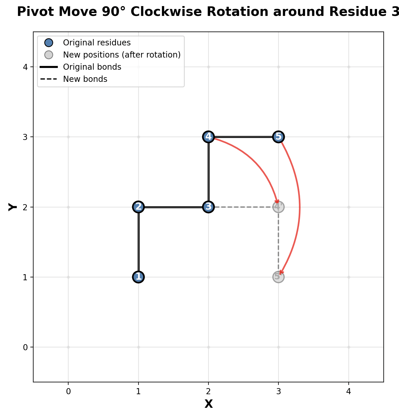
Below is a visualization of a pivot move. It depicts a pivot move for the amino acid at index \(i = 3\) with a 90 degree clockwise rotation. Notice how only residues \(3\) and \(4\) changed positions.
Metropolis-Hastings for HP Model
With our proposal distribution defined, the Metropolis-Hastings algorithm for the HP model becomes:
- Start with an initial valid configuration \(\omega_0\) (e.g., a straight chain)
- At each iteration \(t\):
- Propose a new configuration \(\omega'\) by performing a pivot move on \(\omega_t\)
- Compute the energy difference \(\Delta E = E(s, \omega') - E(s, \omega_t)\)
- Calculate the acceptance probability: \[A(\omega_t, \omega') = \min\left\{1, \frac{e^{-E(s, \omega')/k_B T} \cdot Q(\omega', \omega_t)}{e^{-E(s, \omega_t)/k_B T} \cdot Q(\omega_t, \omega')} \right\} = \min\{1, e^{-\Delta E / k_B T} \cdot R\}\] where \(R = Q(\omega', \omega_t) / Q(\omega_t, \omega')\)
- Accept or reject based on \(A(\omega_t, \omega')\)
- Run for \(T\) iterations until convergence
Notice how the energy calculation simplifies. We only need to count the \(HH\) contacts in \(\omega'\) and \(\omega_t\), which is much faster than computing the full partition function \(Z\). We can write an implementation in python for running this algorithm and visualize how our \(\omega_t\) changes over time for a specific amino acid string. Full disclosure: I’ve generated the following animation by giving Anthropic’s Claude model this algorithm and asking it to write a simulation for the sequence \(s = HPPHPPHHPPHHPPHH\). Click on the play button below to see how the configurations evolve over time.
This should line up with our theoretical result. Recall that our probability distribution \(\pi(\omega) \propto e^{-E(\omega)}\). This function looks something like
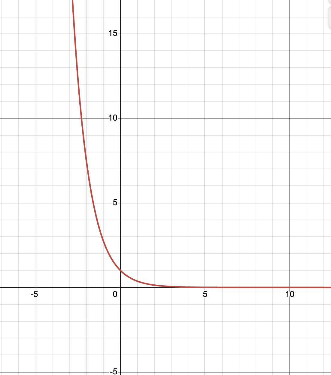
up to different scales and translations. Therefore, the configurations that are most likely under \(\pi\) are ones that minimize the energy function \(E\). Since we defined \(E\) to only count \(HH\) contacts, the configuration that minimizes energy are the ones with the most \(HH\) contacts. This is exactly what we see in the video above! As \(t\) grows, we see that we sample configurations which have more and more \(HH\) contacts. Remember the diagram at the beginning showing how hydrophobic residues cluster together on the inside while polar residues remain on the outside? Now we know exactly why this happens.
Conclusion
The main benefit of this approach is its generality. Whether we’re studying protein folding, sampling from complex Bayesian posteriors, or exploring other high-dimensional probability distributions, the same algorithm can be used. The theoretical guarantees from Markov Chains tells us that given enough time, our samples will be representatives of the true distribution \(\pi\).
Of course, there are practical challenges we didn’t fully address. How many iterations \(T\) do we need before convergence? How do we detect convergence? Can we do better than pivot moves for protein folding? These are active areas of research in computational statistics and biophysics. Variants like Hamiltonian Monte Carlo, Gibbs sampling, and replica exchange methods build on the MH framework to improve convergence rates for specific problem classes. Check out those approaches if this was interesting to you!