Reverse Mode Automatic Differentiation

In this blog post, we will discuss and implement a framework for reverse mode automatic differentiation. This is a useful technique for computing the gradient of a function with respect to its inputs. It is particularly useful in machine learning and deep learning, where we often need to compute the gradient of a loss function with respect to the model parameters.

Why Forward Mode is Not Practical

In the last blog post, I discussed and implemented a framework for forward mode automatic differentiation. It used a new number system called the Dual numbers, denoted as $\mathbb{R}(\epsilon)$, which is an extension of $\mathbb{R}$ with an $\epsilon \neq 0$ such that $\epsilon^2 = 0$. We saw that given an analytic smooth function $f: \mathbb{R}(\epsilon) \to \mathbb{R}(\epsilon)$, if we evaluate it at the dual number $x + \epsilon$, we get the value of the function at $x$ and its derivative at $x$: $$ f(x + \epsilon) = f(x) + f'(x) \epsilon $$ This is a useful property since we can just evaluate the function at a single point to get both the value and the derivative. Turns out, we can extend this approach to work for multi-variable functions of the form $f: \mathbb{R}^n(\epsilon) \to \mathbb{R}(\epsilon)$. The problem is that in multiple variables, we have to compute the gradient, rather than just a single scalar derivative. For functions like $f$ above, the gradient is an $1 \times n$ row vector filled with all the partial derivatives: $$ \nabla f(x) = \begin{bmatrix} \frac{\partial f}{\partial x_1} & \frac{\partial f}{\partial x_2} & \ldots & \frac{\partial f}{\partial x_n} \end{bmatrix} $$

Now, evaluating the function at a dual vector $\vec{x}+ \vec{e_i} \epsilon$ (where $\vec{e_i}$ is the ith standard basis vector) will only give us the value of the function at $\vec{x}$ and the ith coordinate partial derivative $\frac{\partial f}{\partial x_i}$ at $\vec{x}$: $$ f(\vec{x} + \vec{e_i} \epsilon) = f(\vec{x}) + \frac{\partial f}{\partial x_i} \epsilon $$ In order to fully populate the gradient, we need to evaluate the function at $n$ different dual vectors $\vec{x} + \vec{e_i} \epsilon$ for $i = 1, \ldots, n$. If evaluating the function takes $O(C)$ time, then the total time complexity of this approach is $O(nC)$. This is not a problem if $n$ is small, but in practice, $n$ is very large. For example, in deep learning, even simple neural networks can have millions of parameters. So, we need a more efficient way to compute the gradient.

Solution: Reverse Mode Automatic Differentiation

The key idea behind reverse mode automatic differentiation is that any smooth analytic function $f$ can be decomposed into a sequence of elementary operations. This means we can store the intermediate results of the function as we compute it, and then later use these intermediate results to compute the gradient. While forward mode autodiff computes derivatives by propagating the derivative from the input to the output, reverse mode works using the following two steps:

• Forward pass: compute the function value while building a directed acyclic graph (DAG) of the computation.
• Backward pass: traverse the graph in reverse order to compute the gradients, applying the chain rule.

Computation Graph

A computation graph is a directed acyclic graph (DAG) where each node represents an operation or a variable. The edges represent the flow of data between the nodes. The input variables are the leaves of the reversed graph, and the output variable is the root of the reversed graph. For example, consider the function $$ f(x_1, x_2) = x_1 x_2 + \sin(x_1) $$ Its computation graph can be represented as:

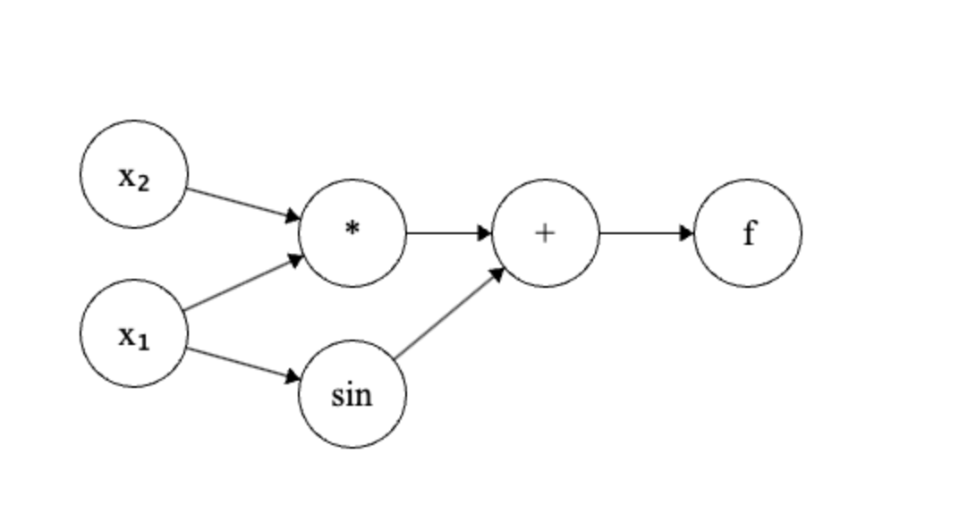
If we let $x_1 = \frac{\pi}{2}$ and $x_2 = 2$, then the forward pass will compute the value of the function as follows:

1. $v_1 = x_1 x_2 = \frac{\pi}{2} \cdot 2 = \pi$.
2. $v_2 = \sin(x_1) = \sin(\frac{\pi}{2}) = 1$.
3. $f(x_1, x_2) = v_1 + v_2 = \pi + 1$.

While computing the function value, we also store the intermediate results $v_1$ and $v_2$ in the graph. The backward pass will compute the gradients as follows:

1. Compute the gradient of the output with respect to the last operation $f = v_1 + v_2$: $$ \frac{\partial f}{\partial v_1} = 1, \quad \frac{\partial f}{\partial v_2} = 1 $$
2. Compute the gradients of the intermediate variables with respect to the output: $$ \frac{\partial v_1}{\partial x_1} = x_2 = 2, \quad \frac{\partial v_1}{\partial x_2} = x_1 = \frac{\pi}{2} $$ $$ \frac{\partial v_2}{\partial x_1} = \cos(x_1) = 0, \quad \frac{\partial v_2}{\partial x_2} = 0 $$
3. Finally, we can compute the gradients of the output with respect to the input variables: $$ \begin{align*} \frac{\partial f}{\partial x_1} &= \frac{\partial f}{\partial v_1} \cdot \frac{\partial v_1}{\partial x_1} + \frac{\partial f}{\partial v_2} \cdot \frac{\partial v_2}{\partial x_1} = 1 \cdot 2 + 1 \cdot 0 = 2 \\ \frac{\partial f}{\partial x_2} &= \frac{\partial f}{\partial v_1} \cdot \frac{\partial v_1}{\partial x_2} + \frac{\partial f}{\partial v_2} \cdot \frac{\partial v_2}{\partial x_2} = 1 \cdot \frac{\pi}{2} + 1 \cdot 0 = \frac{\pi}{2} \end{align*} $$ Therefore, the gradient of $f$ at point $(\frac{\pi}{2}, 2)$ is: $$ \nabla f\left(\frac{\pi}{2}, 2\right) = \begin{bmatrix} 2 & \frac{\pi}{2} \end{bmatrix} $$

Here, we used the chain rule to compute the gradients. As a refresher, multiple variables chain rule states that if $f$ is a function of $v$, and $v$ is a function of $x$, then the derivative of $f$ with respect to $x$ is given by: $$ \frac{\partial f}{\partial x} = \frac{\partial f}{\partial v} \cdot \frac{\partial v}{\partial x} $$ This is the essence of reverse mode automatic differentiation. We compute the function value and the intermediate results in the forward pass, and then we use the chain rule to compute the gradients in the backward pass. More formally, the algorithm for the backward pass can be summarized as follows:

1. Initialize the gradient of the output with respect to itself as 1.
2. Traverse the graph in reverse topological order, and for each node
   1. Compute the gradient of the output with respect to the node using the chain rule.
   2. Compute the gradient of the node with respect to its inputs using the chain rule.
   3. Accumulate the gradients of the inputs using the chain rule.
3. Return the gradients of the output with respect to the inputs.

Note that the cost for the forward pass is $O(C)$, where $C$ is the cost of evaluating the function. In the backward pass, we traverse the graph in reverse order and compute the gradients using the chain rule. Since the graph is a DAG, we can traverse it in $O(C)$ time. Since there is only one output, we can compute the gradients of all inputs in $O(C)$ time. Therefore, the total time complexity of reverse mode automatic differentiation is $O(C)$, which is much better than the $O(nC)$ time complexity of forward mode automatic differentiation!

Implementation in Python

import math
from typing import Union, Set, List, Callable
from collections import defaultdict

class Node:
    """
    A Node in the computation graph that supports reverse mode automatic differentiation.
    """

    def __init__(self, data: float, _children: tuple = (), _op: str = '', label: str = ''):
        self.data = data
        self.grad = 0.0
        self._backward = lambda: None  # Function to compute local gradients, implements chain rule
        self._prev = set(_children) # Parent nodes in the computation graph
        self._op = _op # Operation that produced this node
        self.label = label # Label for the node, debugging purposes

    def __repr__(self):
        return f"Node(data={self.data}, grad={self.grad})"

    def __add__(self, other):
        other = other if isinstance(other, Node) else Node(other)
        out = Node(self.data + other.data, (self, other), '+') # Evaluate the operation and create a new node

        # Save information about this computation's gradient so we can compute the gradients
        # during the backward pass. For addition, the gradient is 1 for both operands since
        # ∂out/∂self = 1 and ∂out/∂other = 1, and so the chain rule gives us:
        # ∂out/∂self * ∂self/∂x + ∂out/∂other * ∂other/∂x = 1 * ∂self/∂x + 1 * ∂other/∂x
        def _backward():
            self.grad += 1.0 * out.grad
            other.grad += 1.0 * out.grad
        out._backward = _backward

        return out

    def __mul__(self, other):
        other = other if isinstance(other, Node) else Node(other)
        out = Node(self.data * other.data, (self, other), '*') # Evaluate the operation and create a new node

        # Again, save information about this computation's gradient.
        # For multiplication, the gradient is given by the product rule:
        # ∂out/∂self = other.data and ∂out/∂other = self.data
        def _backward():
            self.grad += other.data * out.grad
            other.grad += self.data * out.grad
        out._backward = _backward

        return out

    def __pow__(self, other):
        assert isinstance(other, (int, float)), "only supporting int/float powers for now"
        out = Node(self.data**other, (self,), f'**{other}') # Evaluate the operation and create a new node

        # For exponentiation, the gradient is given by the power rule:
        # ∂out/∂self = other * self.data**(other - 1)
        # Note: this is a simplification, in general we would need to consider the chain rule
        # as well, but since we are only supporting int/float powers, we can ignore that.
        def _backward():
            self.grad += other * (self.data ** (other - 1)) * out.grad
        out._backward = _backward

        return out

    def __rmul__(self, other):
        return self * other

    def __truediv__(self, other):
        return self * other**-1

    def __neg__(self):
        return self * -1

    def __sub__(self, other):
        return self + (-other)

    def __rsub__(self, other):
        return other + (-self)

    def exp(self):
        out = Node(math.exp(self.data), (self,), 'exp')

        def _backward():
            self.grad += out.data * out.grad
        out._backward = _backward

        return out

    def log(self):
        out = Node(math.log(self.data), (self,), 'log')

        def _backward():
            self.grad += (1.0 / self.data) * out.grad
        out._backward = _backward

        return out

    def sin(self):
        out = Node(math.sin(self.data), (self,), 'sin')

        def _backward():
            self.grad += math.cos(self.data) * out.grad
        out._backward = _backward

        return out

    def cos(self):
        out = Node(math.cos(self.data), (self,), 'cos')

        def _backward():
            self.grad += -math.sin(self.data) * out.grad
        out._backward = _backward

        return out

    def tan(self):
        out = Node(math.tan(self.data), (self,), 'tan')

        def _backward():
            self.grad += (1.0 / math.cos(self.data)**2) * out.grad
        out._backward = _backward

        return out

    def tanh(self):
        t = math.tanh(self.data)
        out = Node(t, (self,), 'tanh')

        def _backward():
            self.grad += (1 - t**2) * out.grad
        out._backward = _backward

        return out

    def relu(self):
        out = Node(0 if self.data < 0 else self.data, (self,), 'ReLU')

        def _backward():
            self.grad += (out.data > 0) * out.grad
        out._backward = _backward

        return out

    def backward(self):
        """
        Perform reverse mode automatic differentiation to compute gradients
        using the topological order of the computation graph and stored
        backward functions for each node.
        """

        topo = []
        visited = set()

        def build_topo(v):
            if v not in visited:
                visited.add(v)
                for child in v._prev:
                    build_topo(child)
                topo.append(v)

        build_topo(self)

        self.grad = 1.0

        for node in reversed(topo):
            node._backward()

import numpy as np
import matplotlib.pyplot as plt
from mpl_toolkits.mplot3d import Axes3D

def f1(x_node, y_node):
    return x_node * y_node + x_node.sin()

def f2(x_node, y_node):
    return x_node**2 + y_node**2

x_vals = np.linspace(-2, 2, 20)
y_vals = np.linspace(-2, 2, 20)
X, Y = np.meshgrid(x_vals, y_vals)

Z1 = np.zeros_like(X)
grad_x1 = np.zeros_like(X)
grad_y1 = np.zeros_like(Y)

Z2 = np.zeros_like(X)
grad_x2 = np.zeros_like(X)
grad_y2 = np.zeros_like(Y)

for i in range(len(x_vals)):
    for j in range(len(y_vals)):
        x = Node(X[i, j], label=f'x1_{i}_{j}')
        y = Node(Y[i, j], label=f'y1_{i}_{j}')
        z = f1(x, y)
        z.backward()
        Z1[i, j] = z.data
        grad_x1[i, j] = x.grad
        grad_y1[i, j] = y.grad

        x2 = Node(X[i, j], label=f'x2_{i}_{j}')
        y2 = Node(Y[i, j], label=f'y2_{i}_{j}')
        z2 = f2(x2, y2)
        z2.backward()
        Z2[i, j] = z2.data
        grad_x2[i, j] = x2.grad
        grad_y2[i, j] = y2.grad

fig = plt.figure(figsize=(16, 12))

ax1 = fig.add_subplot(221, projection='3d')
ax1.plot_surface(X, Y, Z1, cmap='viridis')
ax1.set_title(r'Plot of $f_1(x,y) = xy + \sin(x)$')
ax1.set_xlabel('X')
ax1.set_ylabel('Y')
ax1.set_zlabel('Z')

ax2 = fig.add_subplot(222, projection='3d')
ax2.quiver(X, Y, Z1, grad_x1, grad_y1, np.zeros_like(Z1), length=0.1, normalize=True)
ax2.set_title(r'Autograd Gradients of $f_1(x,y)$')
ax2.set_xlabel('X')
ax2.set_ylabel('Y')
ax2.set_zlabel('Gradient')

ax3 = fig.add_subplot(223, projection='3d')
ax3.plot_surface(X, Y, Z2, cmap='viridis')
ax3.set_title(r'Plot of $f_2(x,y) = x^2 + y^2$')
ax3.set_xlabel('X')
ax3.set_ylabel('Y')
ax3.set_zlabel('Z')

ax4 = fig.add_subplot(224, projection='3d')
ax4.quiver(X, Y, Z2, grad_x2, grad_y2, np.zeros_like(Z2), length=0.1, normalize=True)
ax4.set_title(r'Autograd Gradients of $f_2(x,y)$')
ax4.set_xlabel('X')
ax4.set_ylabel('Y')
ax4.set_zlabel('Gradient')

plt.tight_layout()
plt.show()